Rigid-body algorithms · LavenderSim

One vector carries rotation and translation

The reference code uses planar spatial motion $v=[\omega_z,v_x,v_y]^\mathsf T$ and force $f=[n_z,f_x,f_y]^\mathsf T$ . A 3×3 spatial inertia maps velocity to momentum and includes the center-of-mass offset.

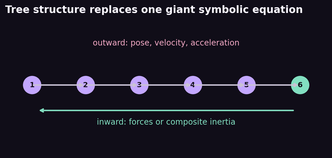
\mathcal I=\begin{bmatrix}I_C+mc^2&0&mc\\0&m&0\\mc&0&m\end{bmatrix}

A motion transform $X_i(q_i)$ maps parent-frame spatial motion to the child joint frame. Because each link depends only on its parent, computation can sweep outward or inward without constructing a global symbolic expression.

Six-link chain with outward and inward recursive passes — RNEA uses one outward and one inward pass. ABA adds a backward articulated-inertia pass followed by an acceleration pass.

Experiment 1: inverse dynamics with RNEA

Inverse dynamics asks for torque given $q,\dot q,\ddot q$ . The Recursive Newton–Euler Algorithm first propagates velocity and acceleration outward, then accumulates link forces inward:

v_i=X_i v_{p(i)}+S_i\dot q_i,\quad a_i=X_i a_{p(i)}+S_i\ddot q_i+v_i\times S_i\dot q_i

f_i=\mathcal I_i a_i+v_i\times^*\mathcal I_i v_i,\qquad \tau_i=S_i^\mathsf T f_i

Experiment 01verified

Compute and replay inverse dynamics

If RNEA computes torque for a desired acceleration, does forward dynamics recover it?

python

torque = rnea(q, qd, desired_qdd, lengths=lengths)
replayed = aba(q, qd, torque, lengths=lengths)
assert np.allclose(replayed, desired_qdd)

For the five-link documented case, the replay error is below 6e-13. Failure modes: forget the negative-gravity base acceleration, transpose a motion transform incorrectly, or use the motion cross product for forces.

Expected result: The command exits successfully and reproduces the numerical or visual relationship described in this card.
Failure modes: Non-finite values, a reversed trend, a failed assertion, or a materially different plot means the assumptions, seed, timestep, build, or backend should be inspected before continuing.

python examples/tutorials/simulation/ch06_rigid_body_algorithms/rigid_body_algorithms.py --quickView source ↗

CRBA constructs the kinetic-energy metric

The Composite Rigid Body Algorithm accumulates each subtree's inertia toward the root. Projecting composite inertia onto pairs of joint motion subspaces fills the symmetric mass matrix:

M_{ij}=S_i^\mathsf T\mathcal I^C_i X_{i\leftarrow j}S_j

Its work grows quadratically because a dense $n\times n$ output itself contains quadratically many values. The test independently generates every mass-matrix column with zero-gravity RNEA and matches CRBA below 2e-13.

ABA avoids forming M for forward dynamics

Dense forward dynamics solves $M\ddot q=\tau-b$ . ABA instead eliminates a leaf joint into its parent's articulated inertia, then recovers accelerations outward. For scalar joints:

U_i=I_i^A S_i,\quad d_i=S_i^\mathsf T U_i,\quad u_i=\tau_i-S_i^\mathsf T p_i^A

\ddot q_i=\frac{u_i-U_i^\mathsf T a_i}{d_i}

Experiment 02verified

Cross-check three independent paths

How do we know a compact recursive implementation is not merely self-consistent?

Tests compare CRBA with RNEA basis columns, ABA with a dense CRBA solve, and RNEA torque replay through both forward paths over seeded random chains of 1, 2, 5, and 12 links.

< 6e-13RNEA ↔ ABA replay

0symmetry error

λmin > 0positive kinetic energy

Failure modes: mutate articulated inertia in the wrong order, omit bias propagation, or divide by a nonpositive projected inertia.

Expected result: The command exits successfully and reproduces the numerical or visual relationship described in this card.
Failure modes: Non-finite values, a reversed trend, a failed assertion, or a materially different plot means the assumptions, seed, timestep, build, or backend should be inspected before continuing.

pytest -q tests/tutorials/test_ch06_rigid_body_algorithms.pyView source ↗

Experiment 3: benchmark 2 through 32 links

Experiment 03verified

Measure work as the chain grows

When do recursive algorithms earn their complexity?

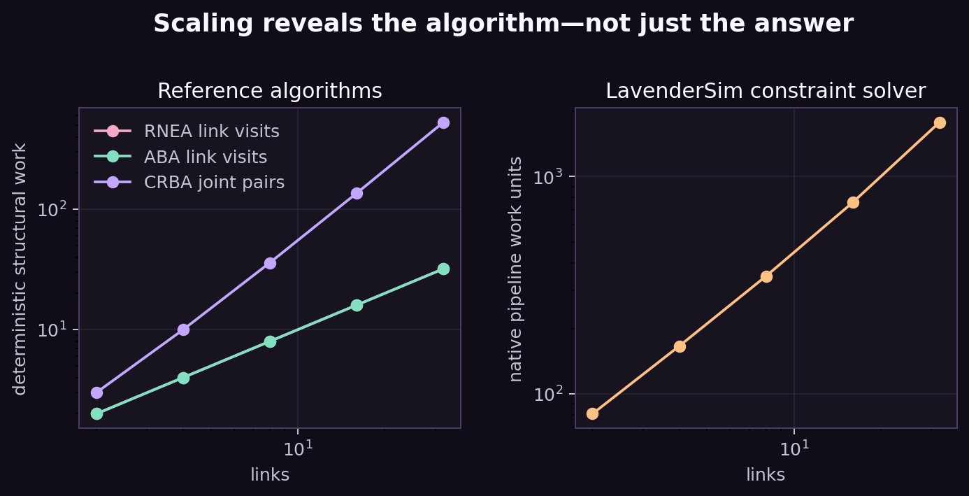
Log scale deterministic work counts for RNEA CRBA ABA and LavenderSim native chain steps — RNEA and ABA visit each link a constant number of times; CRBA must fill joint pairs. The native panel reports public pipeline work units, keeping the committed teaching figure reproducible across machines.

The result manifest stores deterministic work counts: $n$ for RNEA/ABA and $n(n+1)/2$ joint pairs for CRBA. The runnable lab also prints local wall-clock timings; treat those as machine-specific measurements, not universal performance promises.

Expected result: The command exits successfully and reproduces the numerical or visual relationship described in this card.
Failure modes: Non-finite values, a reversed trend, a failed assertion, or a materially different plot means the assumptions, seed, timestep, build, or backend should be inspected before continuing.

python docs-site/scripts/render_tutorial_ch06.pyView source ↗

Experiment 4: contrast the native joint solver

Experiment 04verified

Step Cartesian chains

Why does LavenderSim not call the three algorithms above?

LavenderSim stores body poses and iterates Cartesian joint rows with sequential impulses, then projects residual position error. Chains from 2 to 32 links remain finite; after the smoke rollout, maximum anchor error stays below 8e-7 m.

This solver naturally shares machinery with contacts and closed loops. RNEA/CRBA/ABA instead exploit an open tree whose joints are satisfied by construction. Neither architecture should be described as the other.

Implemented by LavenderSim: substep() iterates joint/contact velocity constraints and then performs position projection.

Expected result: The command exits successfully and reproduces the numerical or visual relationship described in this card.
Failure modes: Non-finite values, a reversed trend, a failed assertion, or a materially different plot means the assumptions, seed, timestep, build, or backend should be inspected before continuing.

python examples/tutorials/simulation/ch06_rigid_body_algorithms/lavendersim_chain_solver.py --quickView source ↗

Paw-check: follow the recursion

Set all velocities to zero and identify which RNEA terms vanish.
Use RNEA basis accelerations to reconstruct M without CRBA.
Count transforms in RNEA and ABA for 100 links.
Add link COM offsets that are not half-length.
Compare dense solve and ABA timing at 64 and 128 links.
Add a closed-loop constraint and explain why the simple tree recursion is no longer sufficient by itself.

What should I be able to say now?

RNEA computes inverse dynamics in linear time, CRBA constructs the dense mass matrix in quadratic time, and ABA computes forward dynamics in linear time without forming that matrix. Spatial vectors make their local recursions uniform. Independent algorithm agreement is a stronger test than one plausible trajectory. LavenderSim currently uses Cartesian sequential impulses instead, trading exact tree-coordinate structure for a compact unified joint-and-contact solver.

By the end, you can…