Constraints · LavenderSim

Turn a geometric promise into a number

A holonomic constraint is a function of configuration that should remain zero:

C(q)=0

For a particle restricted to a circle of radius $r$ :

C(x)=\tfrac12(x^\mathsf T x-r^2)=0

The gradient is the constraint Jacobian $J=\partial C/\partial q$ . Differentiation gives velocity and acceleration conditions:

\dot C=J\dot q=0,\qquad \ddot C=J\ddot q+\dot J\dot q=0

For the circle, $J=x^\mathsf T$ , $\dot C=x\cdot v$ , and $\ddot C=x\cdot a+v\cdot v$ . The runnable test verifies $\dot C$ against a finite difference of $C$ .

Constraint forces live along Jᵀ

Start from unconstrained dynamics $M\ddot q=f$ and add an unknown constraint force:

M\ddot q=f+J^\mathsf T\lambda

Substitution into the acceleration constraint yields the Schur-complement system:

(JM^{-1}J^\mathsf T)\lambda=-\dot J\dot q-JM^{-1}f

$\lambda$ is whatever force magnitude makes the forbidden acceleration vanish. Ideal constraint forces do no work along valid velocity because $(J^\mathsf T\lambda)^\mathsf T\dot q=\lambda^\mathsf T J\dot q=0$ .

Acceleration correctness does not erase position error

Numerical integration can leave $C\ne0$ even when each computed acceleration satisfies $\ddot C=0$ locally. The solver then evolves on the wrong nearby surface.

Baumgarte stabilization asks the residual to behave like a damped oscillator:

\ddot C+2\alpha\dot C+\beta^2 C=0

Projection instead moves the numerical state back onto the manifold after integration. For the circle:

x\leftarrow r\frac{x}{\lVert x\rVert},\qquad v\leftarrow v-x\frac{x\cdot v}{r^2}

Stabilization is force-like and gradual; projection is geometric and immediate. Both can inject or remove energy if tuned or applied carelessly.

Experiment 1: keep a particle on a circle

Experiment 01verified

Compare four constraint treatments

Why does a mathematically correct multiplier still accumulate positional drift?

Particle paths and constraint residuals for unconstrained multiplier Baumgarte and projection methods — The unconstrained tangent escapes. Acceleration-level multipliers bend the path but drift; Baumgarte bounds the error; projection keeps position and velocity constraints at floating-point precision.

> 32unconstrained final |C|

0.003Baumgarte final |C|

< 3e-16projection maximum |C|

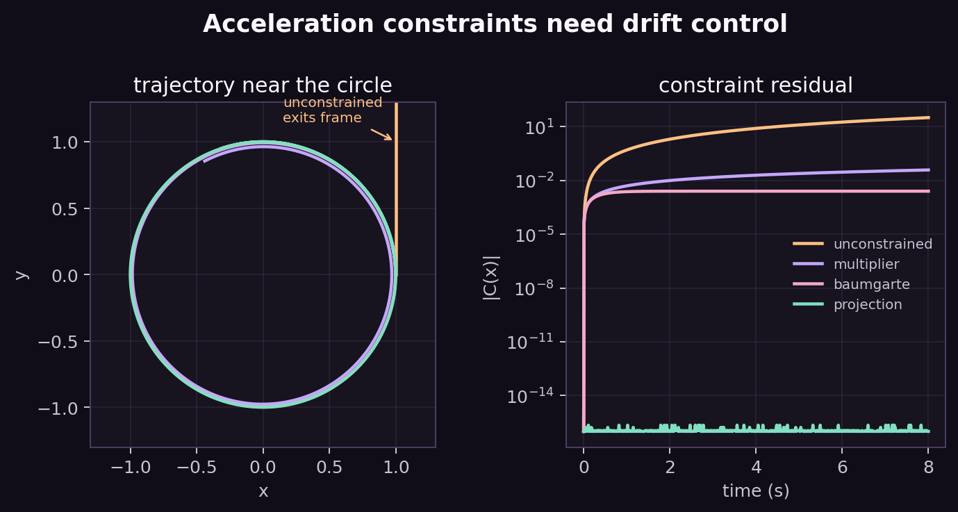
Failure modes: omit the $v\cdot v$ curvature term, choose stabilization gains too large for the timestep, normalize a nearly zero position, or project position without removing radial velocity.

Expected result: The command exits successfully and reproduces the numerical or visual relationship described in this card.
Failure modes: Non-finite values, a reversed trend, a failed assertion, or a materially different plot means the assumptions, seed, timestep, build, or backend should be inspected before continuing.

python examples/tutorials/simulation/ch07_constraints/particle_circle.py --quickView source ↗

A revolute joint is several scalar constraints

In 3D, a revolute joint keeps two anchor points coincident (three scalar rows) and aligns two axes (two independent rows). Rotation about the common axis remains free. A limit adds a unilateral row only when the measured angle crosses its bound.

LavenderSim solves velocity rows repeatedly with sequential impulses, integrates bodies, then performs two positional projection passes. Error-reduction bias turns anchor displacement into a corrective target velocity.

python

diagnostics = sim.constraint_data()
# columns:
# anchor xyz, anchor norm, angular error,
# limit violation, anchor relative speed, coordinate
worst_anchor = diagnostics[:, 3].max()

Experiment 2: inspect the public diagnostics

Experiment 02verified

Perturb a joint by a known amount

Does the engine report the same geometric residual we can calculate by hand?

The test translates a revolute child by $[0.02,0.03,0]$ metres without advancing time. The API reports exactly that anchor-error vector and norm $\sqrt{0.02^2+0.03^2}=0.03606$ within float32 tolerance.

The same eight-column buffer is exported from the shared C++ engine as sim_constraint_data_ptr, bound by native Python, and read by the WebAssembly browser API.

Implemented by LavenderSim: sync_render_data() derives diagnostics from authoritative poses and velocities. constraint_data() exposes a copy or zero-copy NumPy view.

Expected result: The command exits successfully and reproduces the numerical or visual relationship described in this card.
Failure modes: Non-finite values, a reversed trend, a failed assertion, or a materially different plot means the assumptions, seed, timestep, build, or backend should be inspected before continuing.

pytest -q tests/tutorials/test_ch07_constraints.pyView source ↗

Experiment 3: sweep timestep and iterations

Experiment 03verified

Measure native revolute accuracy

Which numerical knobs reduce anchor and axis residuals?

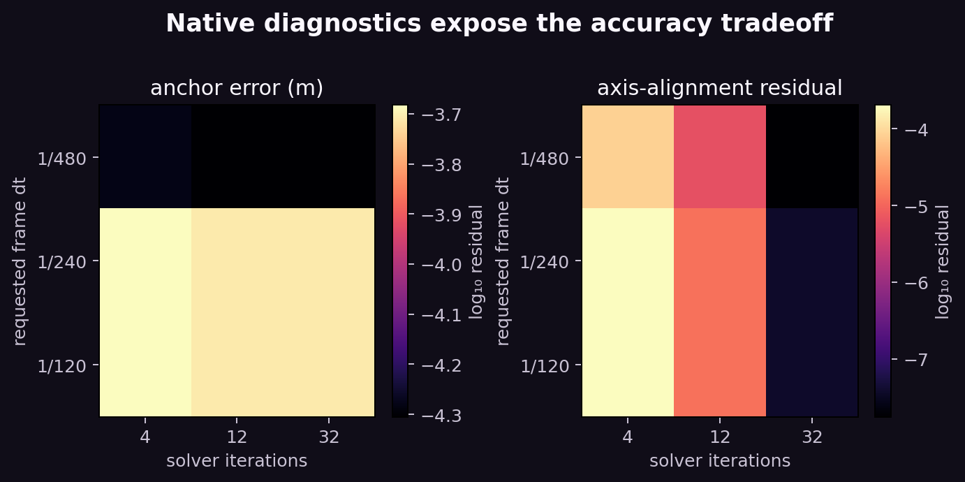
Heatmaps of native anchor and angular residual versus timestep and solver iterations — Increasing iterations from 4 to 32 reduces both residuals under a deliberately inconsistent initial twist. Darker cells are smaller.

LavenderSim internally caps native substeps at 1/240 s. A requested 1/120 s frame therefore becomes two substeps, which explains why its cells resemble 1/240 rather than behaving like one large integration step.

Failure modes: measure only final error and miss an early spike, compare frame dt without knowing internal substeps, or expect more velocity iterations to replace positional projection.

Expected result: The command exits successfully and reproduces the numerical or visual relationship described in this card.
Failure modes: Non-finite values, a reversed trend, a failed assertion, or a materially different plot means the assumptions, seed, timestep, build, or backend should be inspected before continuing.

python examples/tutorials/simulation/ch07_constraints/lavendersim_constraint_sweep.py --quickView source ↗

Paw-check: diagnose the promise

Derive the circle multiplier with a constant external force.
Sweep Baumgarte $\alpha,\beta$ and mark stable and unstable regions.
Plot energy alongside residual for projection.
Trigger a revolute limit and inspect column 5.
Compare a spherical joint's zero angular residual with a fixed joint's orientation residual.
Publish anchor-error vectors as Python-defined browser overlays.

What should I be able to say now?

A constraint is a residual and its Jacobian. Lagrange multipliers generate forces along forbidden directions, but acceleration-level correctness can still drift after numerical integration. Baumgarte feedback and geometric projection control that drift with different energy and tuning tradeoffs. A 3D joint contributes multiple scalar rows, and solver quality should be evaluated with public residuals rather than visual appearance alone.

By the end, you can…