Lagrangian mechanics · LavenderSim

Describe motion with scalar energy

Kinetic energy $T(q,\dot q)$ measures motion; potential energy $V(q)$ measures stored conservative energy. Their difference is the Lagrangian:

\mathcal L(q,\dot q)=T(q,\dot q)-V(q)

For many rigid mechanisms, kinetic energy is quadratic in generalized velocity:

T=\tfrac12\dot q^\mathsf T M(q)\dot q

The mass matrix $M(q)$ is configuration-dependent because changing joint angles rearranges the moving mass. It must be symmetric positive definite for independent coordinates with positive masses.

Euler–Lagrange turns energy into motion

For coordinate $q_i$ and applied generalized force $\tau_i$ :

\frac{d}{dt}\frac{\partial\mathcal L}{\partial\dot q_i}-\frac{\partial\mathcal L}{\partial q_i}=\tau_i

This is not a different physics from Newton's laws. It packages the same mechanics in coordinates that already respect the mechanism's joints, so internal ideal constraint forces disappear from the final coordinate equations.

Experiment 1: derive and integrate a pendulum

Let angle $\theta$ be measured from hanging down, with point mass $m$ , length $l$ , and gravity magnitude $g$ :

T=\tfrac12ml^2\dot\theta^2,\qquad V=mgl(1-\cos\theta)

Applying Euler–Lagrange produces the nonlinear pendulum:

ml^2\ddot\theta+mgl\sin\theta=0

Experiment 01verified

Integrate the nonlinear pendulum

Does an accurate integrator preserve the energy used to derive the equation?

python

def derivative(state):
    theta, omega = state
    return np.array([omega, -(g / length) * np.sin(theta)])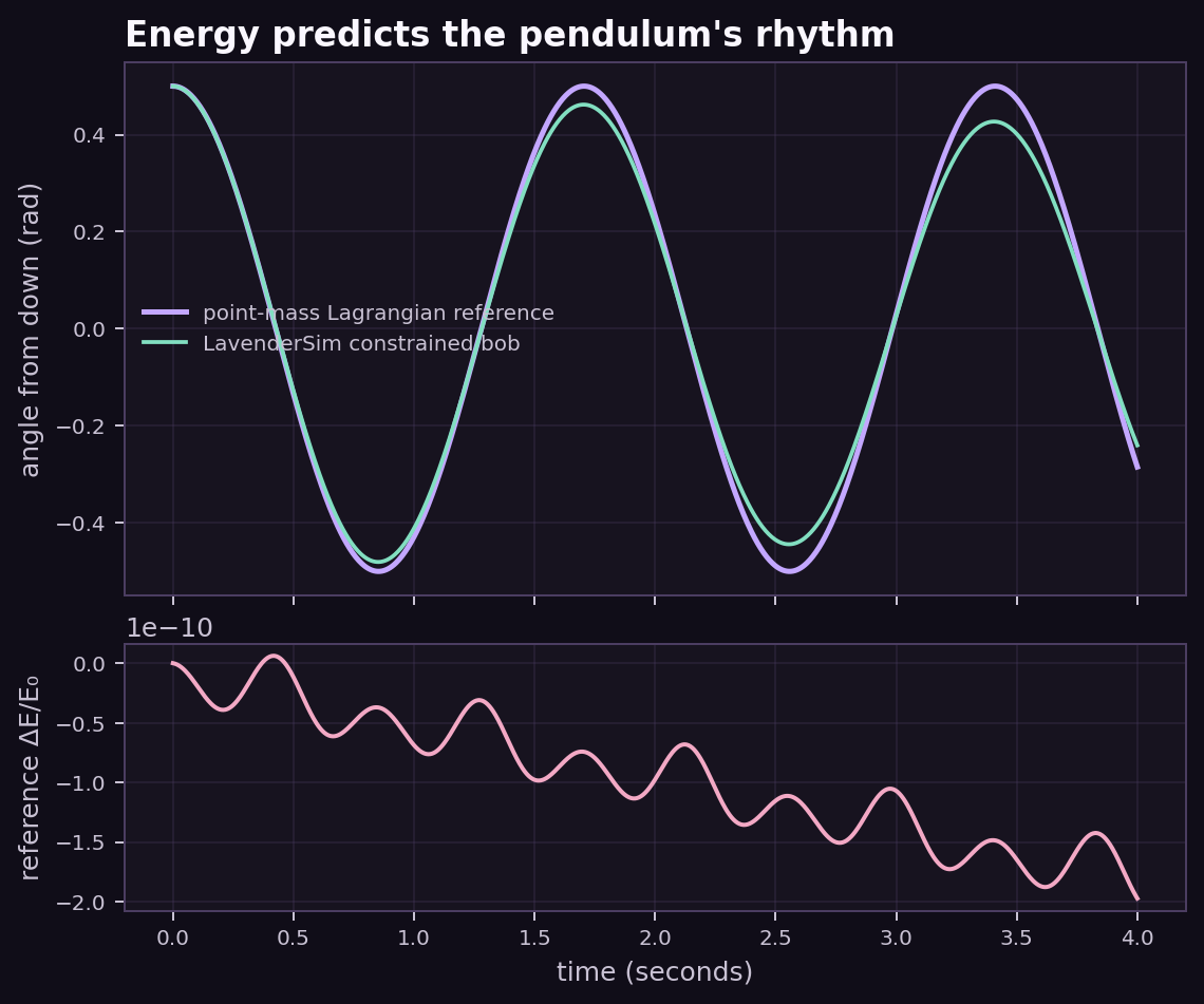

Reference and LavenderSim pendulum angles plus tiny reference energy error — The RK4 reference conserves energy to about 2e-10 relative error. LavenderSim follows the same rhythm with mild damping and a finite rigid bob.

Expected result: oscillation is slightly slower than the small-angle model at finite amplitude. Failure modes: use degrees inside sin, choose potential energy with the wrong sign, or compare numerical energy error to physical damping.

Expected result: The command exits successfully and reproduces the numerical or visual relationship described in this card.
Failure modes: Non-finite values, a reversed trend, a failed assertion, or a materially different plot means the assumptions, seed, timestep, build, or backend should be inspected before continuing.

python examples/tutorials/simulation/ch05_lagrangian_mechanics/lagrangian.py --quickView source ↗

The reusable robot equation

Applying Euler–Lagrange to every coordinate and grouping terms yields:

M(q)\ddot q+C(q,\dot q)+G(q)=\tau

$M$ maps acceleration to inertial torque. $C$ collects velocity-dependent Coriolis and centrifugal terms. $G=\partial V/\partial q$ is the gravity torque. $\tau$ contains applied generalized forces. Some texts use a matrix $C(q,\dot q)\dot q$ ; here $C$ names the already-multiplied vector.

Conventions matter. Gravity signs change with angle definition, and several valid Coriolis-matrix constructions produce the same velocity-force vector. Compare complete equations, not isolated symbols.

Experiment 2: inspect the two-link mass matrix

Experiment 02verified

Sweep inertia through configuration

Can the mass matrix change while remaining a valid kinetic-energy metric?

The reference model places masses at the ends of two massless links. One entry is:

M_{11}=(m_1+m_2)l_1^2+m_2l_2^2+2m_2l_1l_2\cos q_2

The off-diagonal entries encode dynamic coupling: accelerating one joint can require torque at the other.

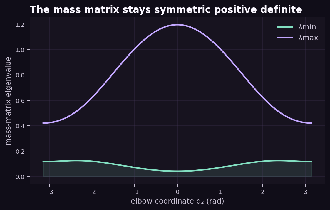
Two positive eigenvalues of a two-link mass matrix across elbow configurations — Both eigenvalues remain positive across the workspace. Symmetry error is numerically zero.

Failure modes: drop one coupling term, use a negative mass, or accidentally build a non-symmetric matrix. The tests sweep the workspace instead of checking one friendly pose.

Expected result: The command exits successfully and reproduces the numerical or visual relationship described in this card.
Failure modes: Non-finite values, a reversed trend, a failed assertion, or a materially different plot means the assumptions, seed, timestep, build, or backend should be inspected before continuing.

pytest -q tests/tutorials/test_ch05_lagrangian_mechanics.pyView source ↗

Experiment 3: cancel gravity without feedback

At rest, $\dot q=0$ and desired $\ddot q=0$ . The necessary holding torque is simply:

\tau_{hold}=G(q)

Experiment 03verified

Plot gravity-compensation torque

Why is one constant motor torque unable to hold an arm everywhere?

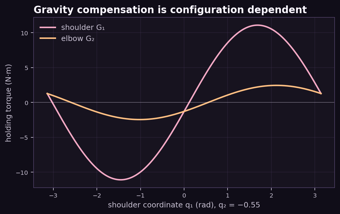
Shoulder and elbow gravity compensation torque versus shoulder angle — The shoulder supports both masses and needs more torque. Both requirements change sign as gravity's moment arm crosses zero.

The executable assertion feeds $G(q)$ into forward dynamics at zero velocity and obtains zero acceleration within 1e-12.

Failure modes: omit the downstream link from shoulder torque, use the controller target instead of measured configuration, or treat gravity compensation as feedback—it is model-based feedforward.

Expected result: The command exits successfully and reproduces the numerical or visual relationship described in this card.
Failure modes: Non-finite values, a reversed trend, a failed assertion, or a materially different plot means the assumptions, seed, timestep, build, or backend should be inspected before continuing.

python examples/tutorials/simulation/ch05_lagrangian_mechanics/lagrangian.pyView source ↗

Forward and inverse dynamics should agree

Inverse dynamics asks for torque given desired acceleration:

\tau=M(q)\ddot q+C(q,\dot q)+G(q)

Forward dynamics asks for acceleration given torque:

\ddot q=M(q)^{-1}\left(\tau-C-G\right)

In code, solve the linear system rather than explicitly forming the inverse:

python

qdd = np.linalg.solve(M, torque - velocity_terms - gravity)
torque = M @ desired_qdd + velocity_terms + gravity

The Chapter 5 test sends $q,\dot q,\ddot q$ through inverse dynamics and back through forward dynamics. The recovered acceleration error is below 1e-15.

Experiment 4: compare a Cartesian constrained pendulum

Experiment 04verified

Measure LavenderSim's pendulum period

Does a Cartesian joint-constraint model recover the generalized-coordinate prediction?

A sphere begins 0.5 rad from downward and is attached to the world by a passive revolute joint. Its angle is measured geometrically from the bob position rather than copied from the reference model.

1.704 snative measured period

1.678 ssmall-angle reference

1.5%relative difference

The finite amplitude increases period; the native bob also has finite rotational inertia, constraint projection, and built-in damping. Agreement in trend and period is the meaningful comparison—not pointwise identity.

Architectural connection: this page derives a generalized-coordinate reference. LavenderSim's substep() instead applies Cartesian forces, solves joint/contact impulses, integrates body poses, and projects constraints.

Expected result: The command exits successfully and reproduces the numerical or visual relationship described in this card.
Failure modes: Non-finite values, a reversed trend, a failed assertion, or a materially different plot means the assumptions, seed, timestep, build, or backend should be inspected before continuing.

python examples/tutorials/simulation/ch05_lagrangian_mechanics/lavendersim_pendulum.py --quickView source ↗

Paw-check: make energy do useful work

Add viscous pendulum damping and verify that energy decreases monotonically.
Derive the physical-pendulum equation by adding center-of-mass inertia.
Numerically differentiate potential energy and compare it with $G(q)$ .
Plot mass-matrix condition number across elbow angle.
Add an external tip force using $\tau=J^\mathsf T F$ .
Vary the native solver iterations and timestep; separate period change from constraint error.

What should I be able to say now?

The Lagrangian is kinetic minus potential energy. Euler–Lagrange converts it into coordinate dynamics. Robot equations organize inertia, velocity coupling, gravity, and applied torque. A valid mass matrix is symmetric positive definite; gravity compensation is configuration-dependent feedforward; and forward/inverse dynamics provide a powerful consistency test. LavenderSim reaches similar physical motion through Cartesian body integration and numerical constraints rather than storing generalized coordinates as its primary state.

Lagrangian mechanics—selectively

By the end, you can…

Describe motion with scalar energy

Euler–Lagrange turns energy into motion

Experiment 1: derive and integrate a pendulum

Integrate the nonlinear pendulum

The reusable robot equation

Experiment 2: inspect the two-link mass matrix

Sweep inertia through configuration

Experiment 3: cancel gravity without feedback

Plot gravity-compensation torque

Forward and inverse dynamics should agree

Experiment 4: compare a Cartesian constrained pendulum

Measure LavenderSim's pendulum period

Paw-check: make energy do useful work