Generalized coordinates

Coordinates are a description, not the mechanism

A degree of freedom is one independent way a system can move. A free rigid body in 3D has six: three translations and three rotations. A revolute joint permits one relative rotation; a prismatic joint permits one relative translation.

Generalized coordinates collect independent configuration variables:

The word “generalized” means the entries need not be Cartesian positions. A coordinate may be a hinge angle, slider distance, or any scalar that locally identifies configuration.

A minimal representation uses exactly one coordinate per degree of freedom. A redundant representation stores extra variables and equations that keep them consistent. For a two-link planar arm:

The 26 scalars are two records of position (3), quaternion (4), linear velocity (3), and angular velocity (3). They are useful for direct collision and rendering, but joint and unit-quaternion constraints make them non-independent.

Joints remove relative motion

Two unconstrained rigid bodies have twelve relative-plus-global degrees of freedom. An ideal revolute joint permits one relative rotation, so it removes five relative directions. A prismatic joint similarly retains one translation and removes the other five relative motions.

A kinematic tree carries transforms outward

A robot description names a root and assigns every non-root link one parent joint. The unique path from root to link lets us multiply transforms in order. For the two-link arm:

Each planar homogeneous transform combines a 2×2 rotation and a translation:

Multiplication order matters. Transforms are functions between named frames; writing the superscripts is a useful defense against accidentally reversing a mapping.

Experiment 1: build forward kinematics

Experiment 01verified

Compose a two-link arm from transforms

How can two joint angles determine every link and site pose?

With lengths $l_1,l_2$, the tip position is:

$$p(q)=\begin{bmatrix}l_1\cos q_1+l_2\cos(q_1+q_2)\\l_1\sin q_1+l_2\sin(q_1+q_2)\end{bmatrix}$$

pythonฅ

elbow = transform_z(q1) @ translation_x(l1)
tip = elbow @ transform_z(q2) @ translation_x(l2)
tip_position = tip[:2, 2]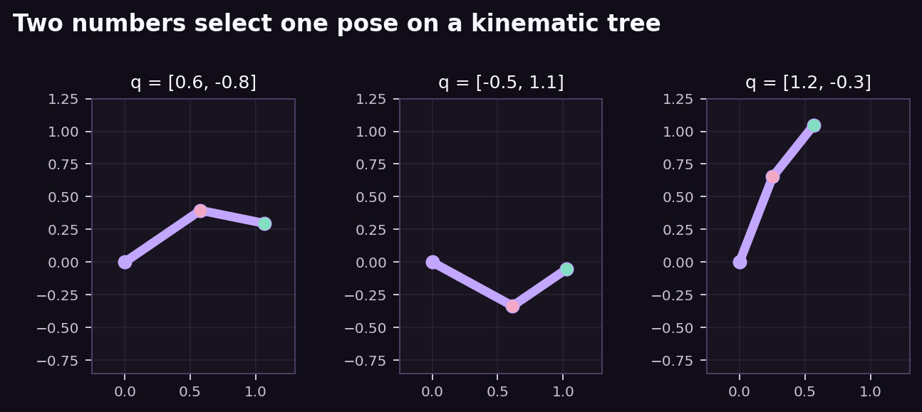

Expected result: at $q=[0,0]$, the tip is $[l_1+l_2,0]$. Failure modes: omit the cumulative $q_1+q_2$, reverse transform order, or confuse a link-center transform with its endpoint.

Expected result

The command exits successfully and reproduces the numerical or visual relationship described in this card.

Failure modes

Non-finite values, a reversed trend, a failed assertion, or a materially different plot means the assumptions, seed, timestep, build, or backend should be inspected before continuing.

python examples/tutorials/simulation/ch04_generalized_coordinates/generalized_coordinates.py --quickView source ↗

Differentiate the tree, not the renderer

The geometric Jacobian maps generalized velocity into tip velocity:

Column $i$ answers: “if only coordinate $q_i$ moves at one unit per second, which way does the tip move?” Upstream joints influence more descendants, which gives tree Jacobians their structure.

Experiment 2: find where q loses leverage

Experiment 02verified

Sweep the elbow through its workspace

When do two independent joints produce only one instantaneous tip direction?

At $q_2=0$ the arm is straight; at $q_2=\pm\pi$ it is fully folded. In both cases the Jacobian columns are parallel and rank falls from two to one.

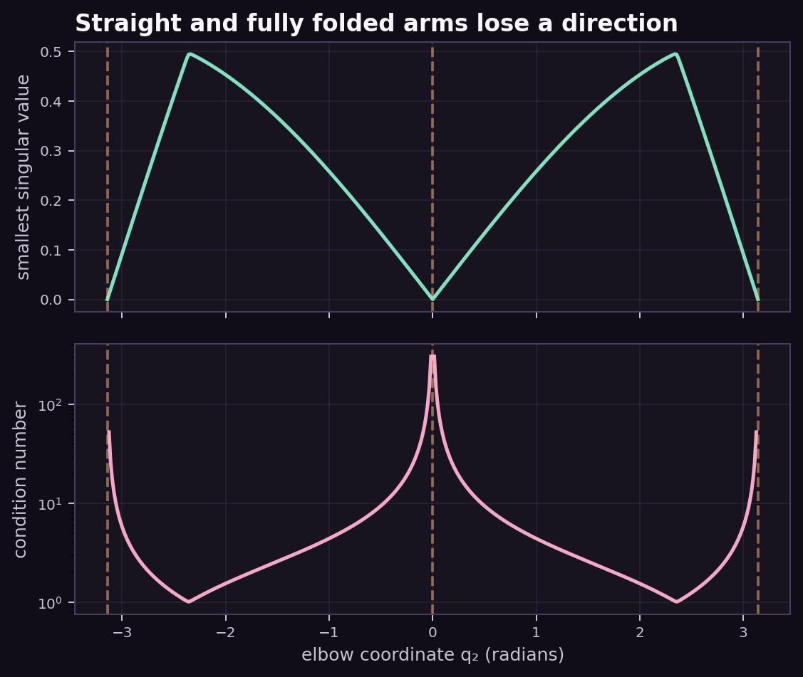
Expected result: rank one at all three marked angles and rank two away from them. Failure modes: use a loose rank tolerance, divide by the zero singular value, or interpret a damped inverse as restoring a physically unavailable motion.

Expected result

The command exits successfully and reproduces the numerical or visual relationship described in this card.

Failure modes

Non-finite values, a reversed trend, a failed assertion, or a materially different plot means the assumptions, seed, timestep, build, or backend should be inspected before continuing.

pytest -q tests/tutorials/test_ch04_generalized_coordinates.pyView source ↗

Experiment 3: map q into LavenderSim

Experiment 03verified

Predict native named-site telemetry

Can minimal-coordinate kinematics reproduce a Cartesian rigid-body scene exactly?

The lab creates a world-fixed base and two revolute links with LavenderSim's scene DSL. It then expands selected $q,\dot q$ values into consistent body positions, quaternions, linear velocities, and angular velocities. The named tip site is measured through the normal native telemetry path.

pythonฅ

scene.revolute(
    "arm.elbow",
    upper,
    forearm,
    anchor=(l1, 0, 0),
    axis=(0, 0, 1),
)
scene.site("arm.tip.site", body=forearm, position=(l2 / 2, 0, 0))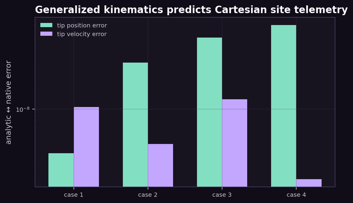

What this verifies: the scene DSL, body-frame site offset, Cartesian body state, and analytic generalized kinematics agree. The lab intentionally imposes a consistent state and does not claim a long dynamic rollout has zero joint-constraint error.

Failure modes to try: give the forearm orientation $q_2$ instead of $q_1+q_2$; omit the moving elbow's velocity; place the site at a world coordinate instead of a body-local offset.

Expected result

The command exits successfully and reproduces the numerical or visual relationship described in this card.

Failure modes

Non-finite values, a reversed trend, a failed assertion, or a materially different plot means the assumptions, seed, timestep, build, or backend should be inspected before continuing.

python examples/tutorials/simulation/ch04_generalized_coordinates/lavendersim_two_link.py --quickView source ↗

Two valid simulator architectures

A generalized-coordinate engine stores $q,\dot q$ for a kinematic tree and derives link poses. Joint constraints are satisfied by construction, while contacts and closed loops still introduce constraints.

LavenderSim currently stores every body's Cartesian pose and twist. Its revolute solver preserves a common anchor, aligns two axes, and leaves rotation about that axis free. This makes the compact engine and collision pipeline direct, but articulation accuracy depends on timestep, projection, and solver iterations.

Paw-check: choose coordinates deliberately

1. Add a third link. Write its tip transform before expanding the trigonometry.
2. Derive the two-link Jacobian by treating each revolute column as $\hat z\times(p_{tip}-p_{joint})$.
3. Plot the reachable annulus and identify its inner and outer radii.
4. Add a prismatic first joint and decide its coordinate unit and Jacobian column.
5. Step the native chain dynamically instead of imposing state. Sweep solver iterations and measure anchor error.
6. Explain why a closed four-bar linkage cannot be represented by a simple tree without an extra closure constraint.