Simulation architecture

One public step contains several physical substeps

An RL policy commonly acts at 60 Hz, but LavenderSim limits the native physics timestep to 1/240 s. One control step therefore performs four physical substeps. The control is held while forces, collision detection, constraint solving, integration, correction, and sensing repeat. At the end, telemetry is copied into flat buffers for Python or JavaScript.

Here $x_k$ is complete simulator state, $u_k$ is the command held for the control interval, $F$ is one substep, and $N=4$ at 60 Hz with 240 Hz physics. Changing the ordering changes $F$ even when every individual formula stays the same.

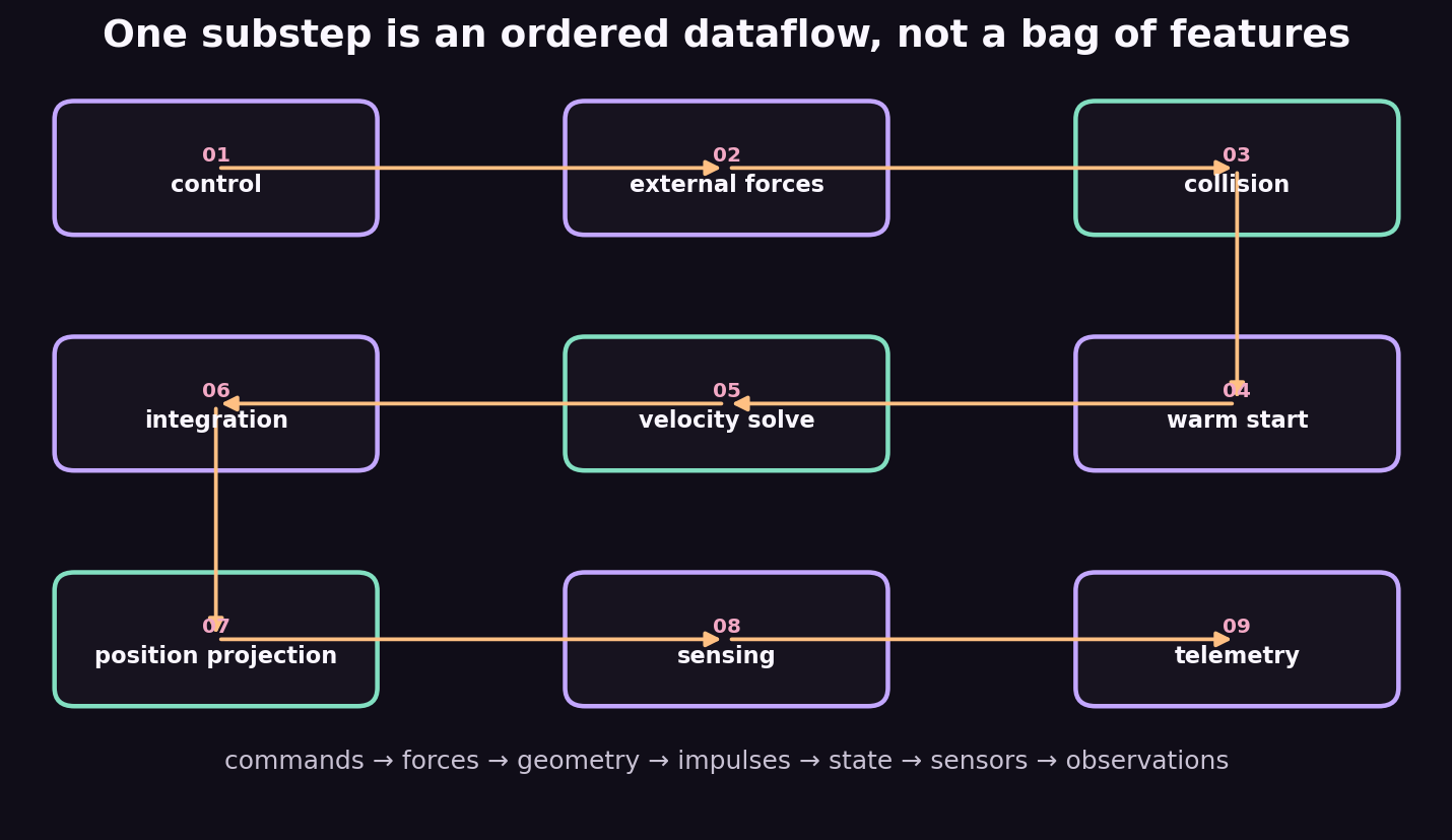
Experiment 1: single-step the architecture

The reference lab writes every read and write explicitly. Select a stage below and ask: what would become one-step stale if it moved earlier?

for stage in pipeline:
    event = stage(state, control, dt)
    trace.append({"reads": event.reads,
                  "writes": event.writes})

Experiment 2: profile work, not your intuition

Native timing is opt-in because clocks perturb tiny workloads. Calling set_profiling(True) fills the third trace column with elapsed microseconds. The second column is a deterministic work counter—bodies, candidate pairs, solver row-visits, samples, or copied records depending on the stage. Work units compare runs; they are deliberately not interchangeable durations.

Experiment 02verified

Profile the quadruped pipeline

Which stages grow with articulated contact?

pythonฅ

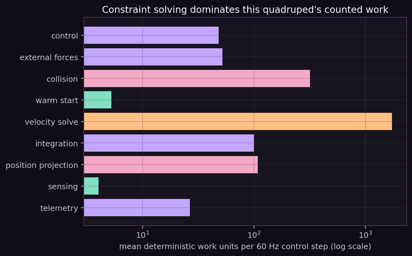
env.sim.set_profiling(True)
observation, reward, terminated, truncated, info = env.step(action)
trace = env.sim.pipeline_trace()
# columns: stage_id, work_units, native_microseconds

Failure modes: benchmark a debug build, infer time from work units, include process startup, compare different scenes, or report one sample without distribution or hardware context.

Expected result

The command exits successfully and reproduces the numerical or visual relationship described in this card.

Failure modes

Non-finite values, a reversed trend, a failed assertion, or a materially different plot means the assumptions, seed, timestep, build, or backend should be inspected before continuing.

python examples/tutorials/simulation/ch12_simulation_architecture/lavendersim_pipeline.py --include-timingView source ↗

Experiment 3: one contract, two backends

The browser build runs the same C++ source compiled to freestanding WebAssembly. It exposes stage IDs and work units, but records zero in the timing column because the module has no host clock import. Browser wall-clock profiling belongs around the JavaScript call; semantic engine parity belongs inside the trace.

Experiment 03verified

Compare a resting sphere in native and WASM

Do both builds execute the same stage contract?

9 / 9stage IDs equal

0maximum body error

0maximum solver error

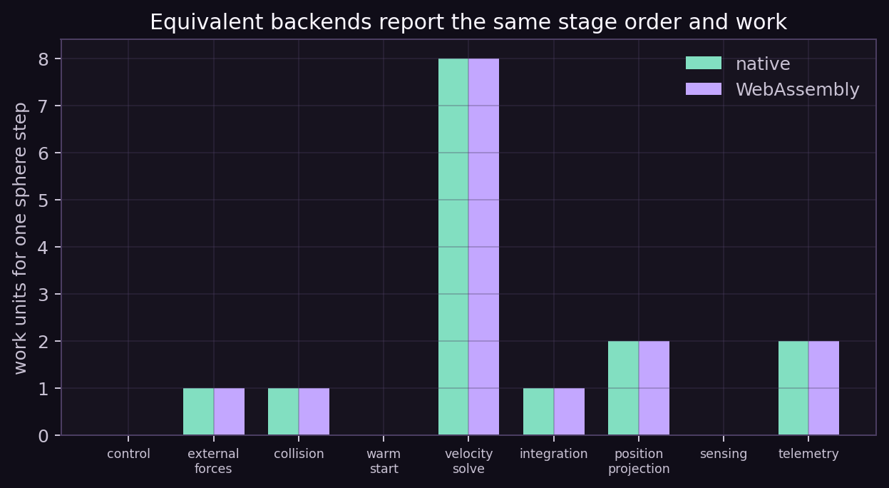
Failure modes: compare native time with a missing WASM clock, verify only exported symbol names, use different scene defaults, or generalize one exact trace to all hardware and all trajectories.

Expected result

The command exits successfully and reproduces the numerical or visual relationship described in this card.

Failure modes

Non-finite values, a reversed trend, a failed assertion, or a materially different plot means the assumptions, seed, timestep, build, or backend should be inspected before continuing.

node scripts/check_wasm_exports.mjsView source ↗

Experiment 4: rewind, replay, branch

A snapshot turns simulation into an experiment tree. Save at state $x_t$, apply action sequence $U$, restore, and repeat $U$ to test determinism. Restore again and apply $U'$ to isolate the action's causal effect.

Experiment 04verified

Replay one force and branch to its opposite

Can serialized state reproduce the same trajectory before a counterfactual diverges?

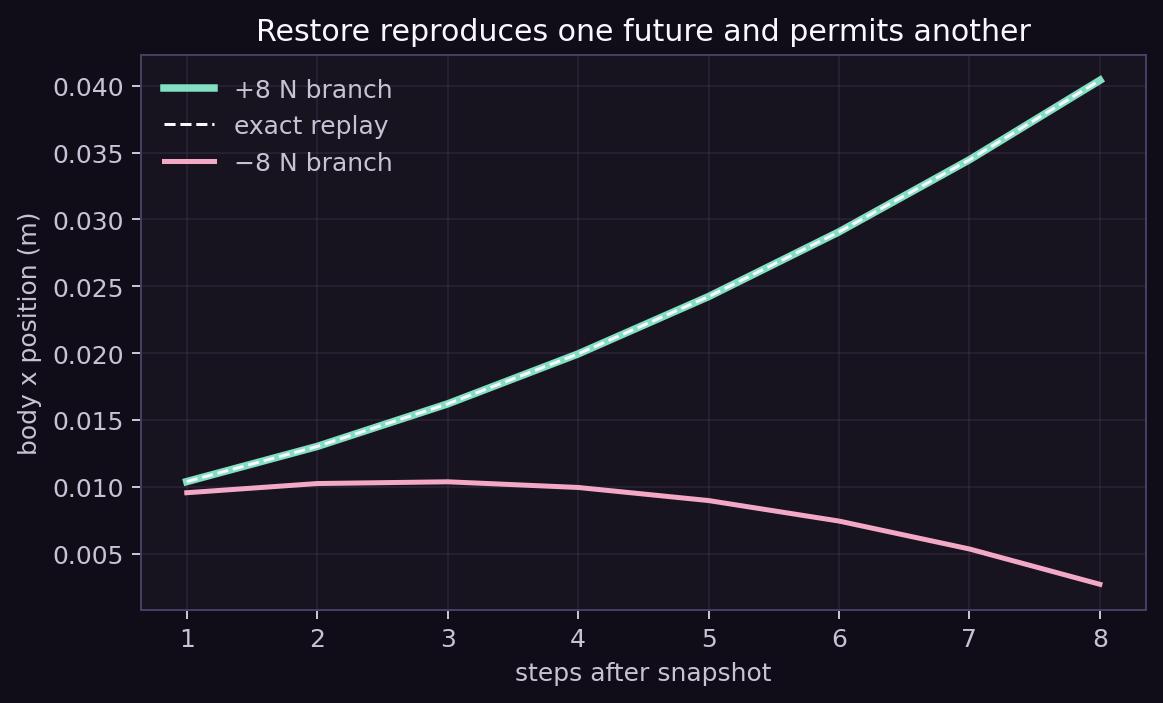
The current snapshot covers bodies, joints, controls, actuator activation, Python sensor pipeline state and RNG, solver controls, task state, and time. The demonstrated exact replay intentionally avoids persistent contacts; contact-cache and native sensor-filter serialization remain a boundary to test before claiming arbitrary contact-rich bitwise replay.

Expected result

The command exits successfully and reproduces the numerical or visual relationship described in this card.

Failure modes

Non-finite values, a reversed trend, a failed assertion, or a materially different plot means the assumptions, seed, timestep, build, or backend should be inspected before continuing.

pytest -q tests/tutorials/test_ch12_simulation_architecture.pyView source ↗

Experiment 5: make one environment become 32

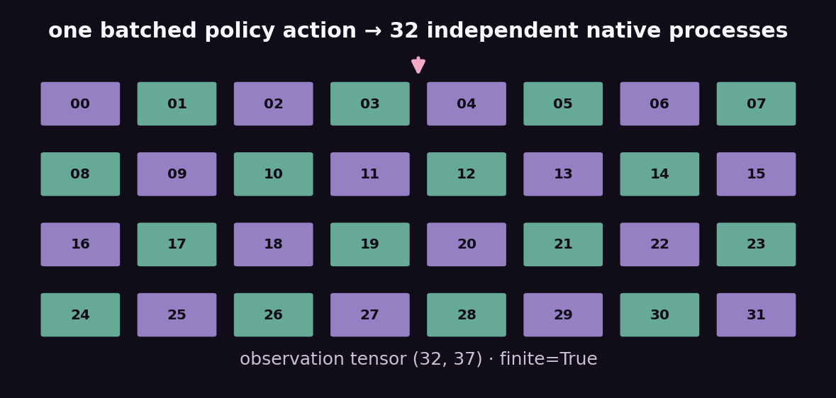
PPO needs many decorrelated transitions. ProcessVectorEnv creates 32 independent registry instances, sends a batch of actions, then stacks their flat observations and rewards. It is 32 copies of one registered task—not 32 different task types.

Experiment 05verified

Roll out 32 registry-created workers

Does the environment contract remain finite and rectangular across processes?

pythonฅ

with ProcessVectorEnv(32, task="QuadrupedCommand-v0",
                          control_hz=60, horizon_seconds=3) as env:
    obs = env.reset(seed=12)       # (32, 37)
    obs, reward, done, info = env.step(actions)

Failure modes: reuse one RNG stream in every worker, forget to close processes, silently flatten the environment axis, launch a browser per worker, or confuse simulator throughput with PPO sample quality.

Expected result

The command exits successfully and reproduces the numerical or visual relationship described in this card.

Failure modes

Non-finite values, a reversed trend, a failed assertion, or a materially different plot means the assumptions, seed, timestep, build, or backend should be inspected before continuing.

python examples/tutorials/simulation/ch12_simulation_architecture/lavendersim_pipeline.pyView source ↗

Capstone: follow one quadruped action end to end

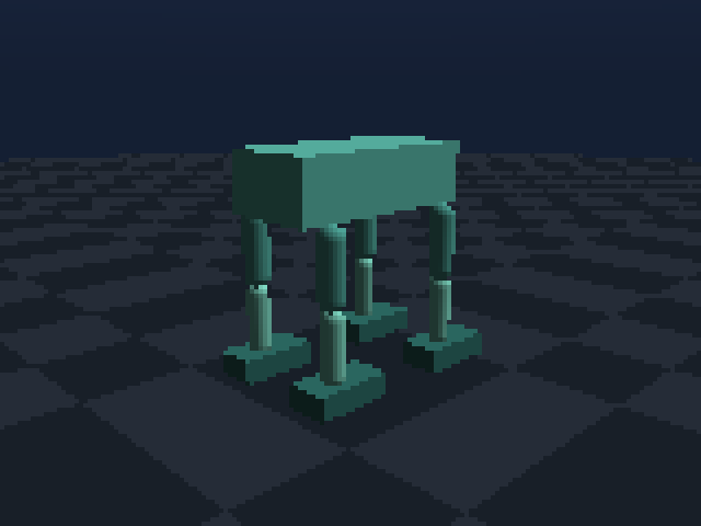
1. The environment samples a body-relative planar direction and speed, then assembles 37 proprioceptive and command values.
2. A controller or policy emits 12 joint actions at 60 Hz.
3. Actuator forces, gravity, damping, and user wrenches update four 240 Hz substeps.
4. Collision manifolds and joint rows feed the warm-started sequential-impulse solve.
5. Velocity integration and position projection produce the physical state sampled by IMU and joint sensors.
6. The task computes command-tracking reward; telemetry and overlays can be published to the Python-controlled browser UI.
7. The process vectorizer repeats that contract across 32 isolated workers for PPO.

Paw-check: reason across stage boundaries

1. Move sensing before projection in the toy lab. Which quantities become inconsistent?
2. Profile a contact-free scene and explain the changed work vector.
3. Add host-side browser timing around sim_step without changing the backend parity contract.
4. Snapshot a noisy delayed sensor and prove its replay behavior.
5. Increase physics frequency while holding 60 Hz control constant; predict work and stability changes.
6. Profile 32 workers without including process creation in per-step latency.
7. Replace the deterministic quadruped gait with a checkpoint and keep the engine assertions unchanged.