Constraint solvers · LavenderSim

Every constraint row talks through the bodies

Start with unconstrained velocity $v^*$ and apply constraint impulses $J^T\lambda$ through inverse mass:

v^+=v^*+M^{-1}J^T\lambda

If a bilateral constraint asks for $Jv^+=b$ , substitution gives a system in constraint space:

\underbrace{JM^{-1}J^T}_{A}\lambda=b-Jv^*

$A$ is the effective-mass matrix. Its diagonal tells how one row responds to its own impulse; off-diagonal terms encode coupling through shared bodies. A six-block stack is not six unrelated floor contacts—the bottom impulse must support everything above it.

Experiment 1: solve exactly or improve cheaply

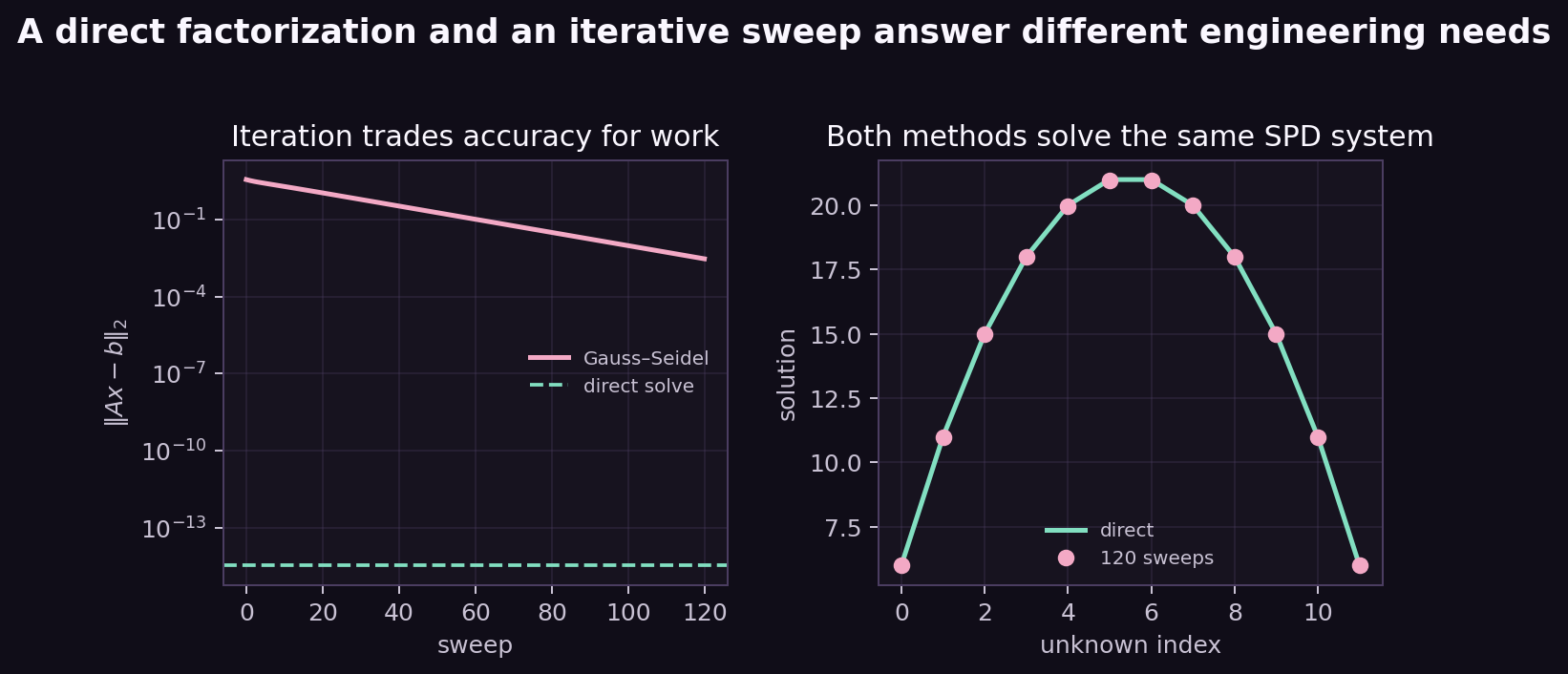
A direct method factors $A$ and solves for every impulse together. For a dense $n\times n$ system, generic factorization costs about $O(n^3)$ , though sparsity and structure can help. Gauss–Seidel updates one row using the newest preceding values:

\lambda_i\leftarrow\lambda_i+\frac{b_i-A_{i:}\lambda}{A_{ii}}

One sweep is cheap and interruptible. It is not “an approximate equation”; it is an algorithm whose answer depends on condition number and allotted sweeps.

Experiment 01verified

Compare a direct SPD solve with Gauss–Seidel

How does a fixed iteration budget differ from a factorization?

Residual history and solution comparison for direct and Gauss Seidel SPD solves — The direct solve reaches floating-point residual immediately after factorization. Gauss–Seidel approaches the same solution incrementally and can stop at any budget.

python

for sweep in range(iterations):
    for i in range(n):
        correction = (b[i] - A[i] @ impulse) / A[i, i]
        impulse[i] += correction

Failure modes: compare only final positions, use a singular diagonal, assume every SPD system converges at the same rate, or call a low residual “exact physics.”

Expected result: The command exits successfully and reproduces the numerical or visual relationship described in this card.
Failure modes: Non-finite values, a reversed trend, a failed assertion, or a materially different plot means the assumptions, seed, timestep, build, or backend should be inspected before continuing.

python examples/tutorials/simulation/ch11_constraint_solvers/constraint_solvers.py --quickView source ↗

Experiment 2: contact turns the solve into inequalities

A bilateral row allows impulses of either sign. Normal contact must obey:

w=A\lambda-b\ge0,qquad\lambda\ge0,qquad\lambda^Tw=0

This is a linear complementarity problem (LCP). When $A$ is symmetric positive semidefinite, it is also the optimality condition of a constrained quadratic program:

\min_{\lambda\ge0}\frac12\lambda^TA\lambda-b^T\lambda

Projected Gauss–Seidel (PGS) performs the scalar update, then projects $\lambda_i\leftarrow\max(0,\lambda_i)$ . The projection enforces no-pulling impulses throughout iteration.

Experiment 02verified

Solve a toy stack LCP

Do nonnegative impulse and nonnegative slack approach complementary values?

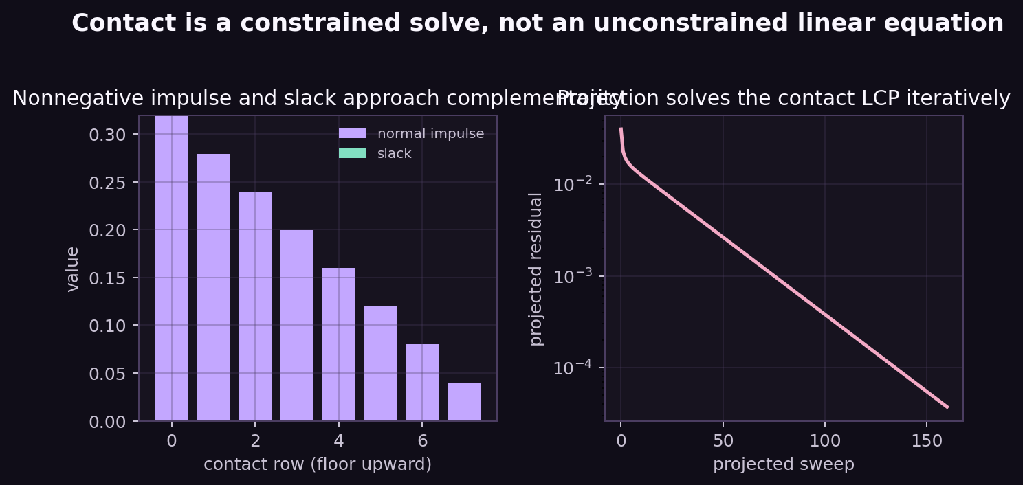
Contact impulses slack and projected residual across PGS sweeps — Eight coupled stack contacts converge toward positive support impulses and nearly zero active-contact slack. The projected residual measures the change another legal update would make.

A useful projected fixed-point residual is:

r_p=\left\lVert\lambda-\Pi_{\lambda\ge0}\left(\lambda-(A\lambda-b)\right)\right\rVert

Failure modes: solve $A\lambda=b$ then clamp once, use ordinary residual alone at an inactive contact, permit negative normal impulses during a sweep, or confuse complementarity with penetration correction.

Expected result: The command exits successfully and reproduces the numerical or visual relationship described in this card.
Failure modes: Non-finite values, a reversed trend, a failed assertion, or a materially different plot means the assumptions, seed, timestep, build, or backend should be inspected before continuing.

pytest -q tests/tutorials/test_ch11_constraint_solvers.pyView source ↗

Sequential impulses are matrix-free PGS

A rigid-body engine need not assemble dense $A$ . For one row, it computes relative velocity, scalar effective mass $A_{ii}$ , and a projected impulse increment; applying that impulse to bodies immediately updates velocities seen by later rows. This is the sequential impulse view of PGS.

LavenderSim visits all joint rows, then all contact rows, repeatedly. Each contact update solves normal response, a two-dimensional friction-disk projection, and angular patch friction. The current engine uses a fixed 4–64 sweep budget rather than an early-exit tolerance.

Implemented by LavenderSim: substep() performs the repeated joint/contact ordering. solve_contact_velocity() applies projected normal and friction impulses without forming a global matrix.

Experiment 3: order and memory are algorithm inputs

Gauss–Seidel is order dependent because later rows see newer velocities. In a floor-to-top stack, processing the bottom row first propagates support upward sooner than the reverse order. Graph coloring and parallel Jacobi-style updates trade some propagation speed for parallelism.

Warm starting maps persistent contacts to the previous step's impulses and applies them before iteration. If the scene changes slowly, this is an excellent initial guess. If matching is wrong, stale impulses can hurt.

Experiment 03verified

Reorder a stack and warm its next solve

How much accuracy can order and initialization buy without adding sweeps?

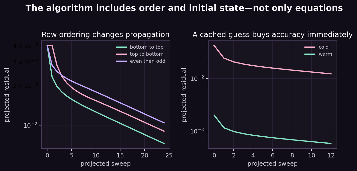
Projected residual histories by contact ordering and cold versus warm initial impulse — Bottom-to-top propagation wins this stack's fixed budget. A small load change starts roughly twenty times closer when initialized with the previous exact impulses.

There is no universally best order. Articulated joints, shocks, stacks, islands, and parallel hardware create different priorities. Always report the order used by a benchmark.

Expected result: The command exits successfully and reproduces the numerical or visual relationship described in this card.
Failure modes: Non-finite values, a reversed trend, a failed assertion, or a materially different plot means the assumptions, seed, timestep, build, or backend should be inspected before continuing.

python examples/tutorials/simulation/ch11_constraint_solvers/constraint_solvers.pyView source ↗

Experiment 4: expose convergence in the real engine

LavenderSim now publishes eight solver values for the final substep: configured iterations, warm-start flag, contact count, cache matches, initial/final projected normal-impulse residual, and initial/final normal-velocity violation. The residual asks how much one more projected normal update would change an impulse.

python

scene = Scene("stack", solver_iterations=8, warm_start=True)
observation, *_ = sim.step()
print(observation["solver"])

sim.set_solver_iterations(32)
sim.set_warm_start(False)

Experiment 04verified

Sweep 4 to 64 native iterations

Do public residuals predict visible stack quality?

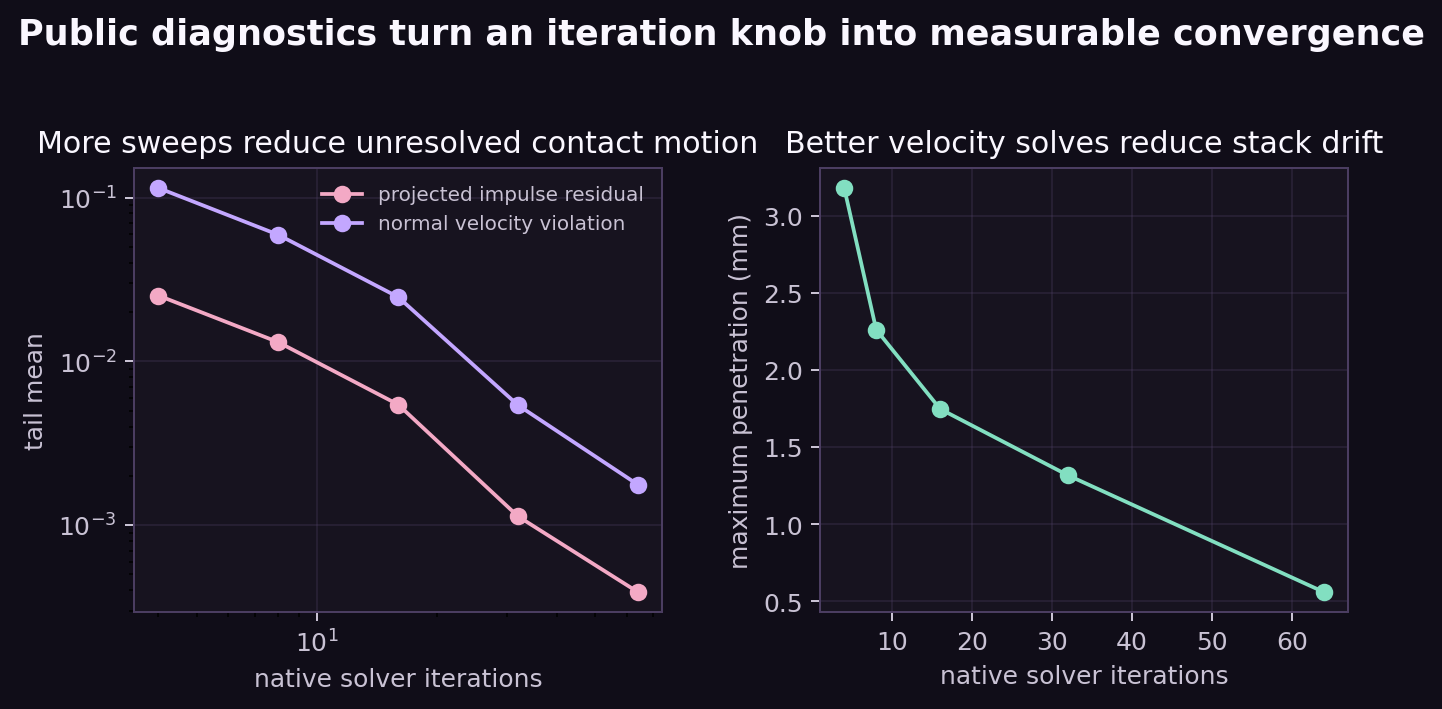
Native projected residual velocity violation and penetration across solver iterations — At 64 cold sweeps, tail residual is about 45× smaller than at 4; velocity violation and maximum penetration fall with it.

The diagnostic is intentionally scoped: it measures projected normal-contact convergence, not a complete norm over joint, tangent, torsion, and position-projection rows. Its value is causal comparison under a fixed scene.

Expected result: The command exits successfully and reproduces the numerical or visual relationship described in this card.
Failure modes: Non-finite values, a reversed trend, a failed assertion, or a materially different plot means the assumptions, seed, timestep, build, or backend should be inspected before continuing.

python examples/tutorials/simulation/ch11_constraint_solvers/lavendersim_solver_sweep.py --quickView source ↗

Experiment 05verified

Toggle native warm starting

Can four sweeps support a stack when persistent contacts supply a good first guess?

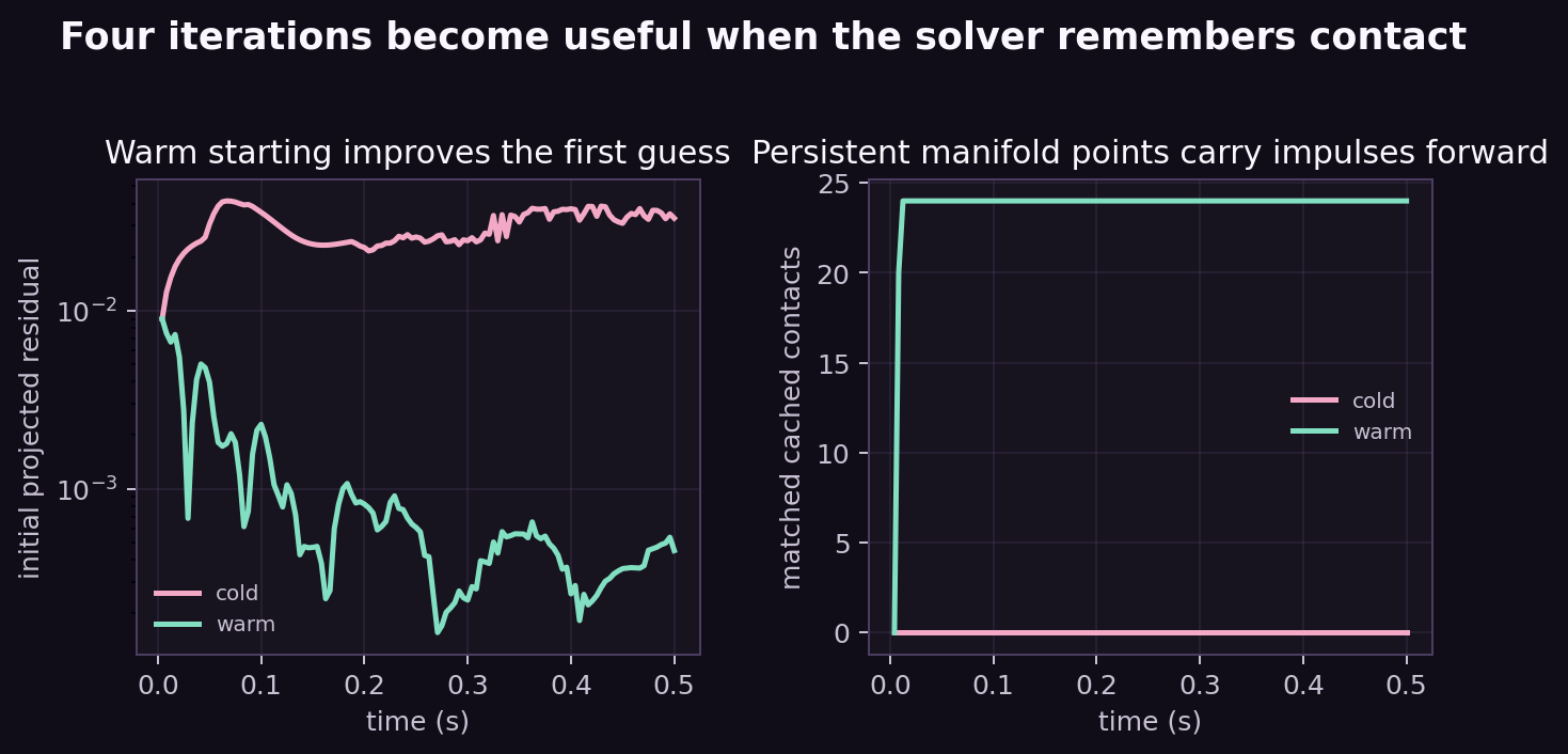
Native cold and warm initial residual plus matched contact counts over time — Cold starts match no cached contacts. Warm starts settle to 24 matched manifold points and reduce the four-sweep initial residual by roughly two orders of magnitude.

The setting and the eight-value buffer are equivalent in native and WebAssembly builds. Solver iterations and warm-start mode are also included in Python snapshot/restore state.

Backend parity: check_wasm_exports.mjs creates persistent contact, proves a cache match, disables warm starting, and verifies the WebAssembly diagnostic changes to zero matches.

Expected result: The command exits successfully and reproduces the numerical or visual relationship described in this card.
Failure modes: Non-finite values, a reversed trend, a failed assertion, or a materially different plot means the assumptions, seed, timestep, build, or backend should be inspected before continuing.

node scripts/check_wasm_exports.mjsView source ↗

Paw-check: budget error deliberately

Derive $A=JM^{-1}J^T$ for two particles joined by one distance row.
Implement Jacobi iteration and compare its parallel-friendly convergence.
Construct a case where top-to-bottom contact order wins.
Add friction bounds to the toy contact QP.
Stop PGS on a tolerance and compare variable cost with a fixed budget.
Disable warm starting midway through the native stack and plot the transient.
Design a diagnostic that also includes tangent and joint rows without mixing incompatible units carelessly.

What should I be able to say now?

Constraint impulses solve a coupled effective-mass system. Direct methods factor that system; Gauss–Seidel and sequential impulses improve one row at a time. Unilateral contact creates complementarity and requires projection. Row order and warm-start state materially affect a fixed iteration budget. Residuals, tolerances, and iteration counts are different quantities, and public diagnostics are the right way to compare them.

By the end, you can…