Linear algebra for mechanics

A vector needs a meaning and a frame

The array [1, 0, 0] is not yet a physical statement. Is it a point, a direction, a velocity, or a force? Is it expressed in the robot body frame or the world frame? Correct arithmetic begins by answering both questions.

The dot product measures alignment:

The cross product produces a vector perpendicular to two inputs. Mechanics uses it for torque and point velocity:

It is often useful to write the cross product as matrix multiplication:

def skew(vector):
    x, y, z = vector
    return np.array([
        [0, -z,  y],
        [z,  0, -x],
        [-y, x,  0],
    ], dtype=float)

Points translate; free vectors only rotate

A rigid transform contains a rotation $R$ and translation $t$. A local point includes both:

A direction, angular velocity, or force has no location, so translation does not apply:

A valid rotation satisfies $R^\mathsf{T}R=I$ and $\det R=1$. Its inverse is therefore its transpose. The inverse rigid transform is:

Linear systems and quadratic forms

Simulation repeatedly solves equations that can be organized as:

$A$ may encode inertia, constraint coupling, or a local approximation to nonlinear dynamics. We normally solve the system with a factorization instead of explicitly forming $A^{-1}$. Explicit inversion does more work, hides exploitable structure, and often magnifies numerical error.

A quadratic form maps a direction to a scalar:

When symmetric $A$ is positive definite, $x^\mathsf{T}Ax>0$ for every nonzero $x$. Mass and inertia matrices should have this property: every nonzero velocity stores positive kinetic energy.

Experiment 1: find the principal axes

Experiment 01verified

Rotate and diagonalize an inertia tensor

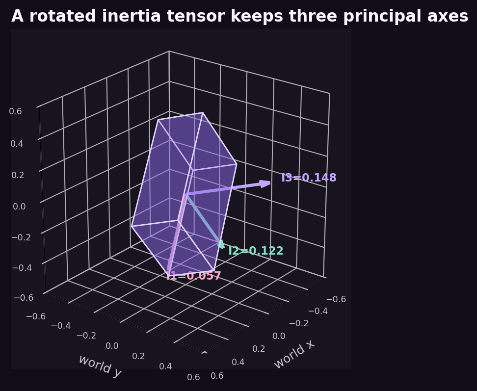
If a box is rotated in the world, did its physical resistance to rotation change—or only its coordinates?

A uniform box aligned with its body axes has diagonal inertia:

$$I_B=\frac{m}{12}\operatorname{diag}(h^2+d^2,\;w^2+d^2,\;w^2+h^2)$$

Expressed in world coordinates, the same tensor becomes:

$$I_W=R_{WB}I_BR_{WB}^{\mathsf T}$$

The eigenvectors of $I_W$ point along the rotated principal axes. The eigenvalues are the principal moments and remain unchanged by rotation.

det R = 1proper rotation

3 positive λpositive-definite inertia

I = VΛVᵀeigen reconstruction

Expected result

The command exits successfully and reproduces the numerical or visual relationship described in this card.

Failure modes

Non-finite values, a reversed trend, a failed assertion, or a materially different plot means the assumptions, seed, timestep, build, or backend should be inspected before continuing.

python examples/tutorials/simulation/ch02_linear_algebra/linear_algebra.py --quickView source ↗

Experiment 2: differentiate a two-link arm

For link lengths $l_1,l_2$ and joint angles $q_1,q_2$, the planar tip is:

The Jacobian contains the derivative of every output coordinate with respect to every input coordinate:

It maps joint velocity to instantaneous Cartesian tip velocity:

analytic = two_link_jacobian(q)
numeric = finite_difference_jacobian(two_link_tip, q)

assert np.allclose(analytic, numeric, atol=2e-10)

Experiment 3: lose a motion direction

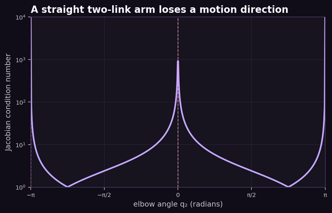
A singular value measures how strongly a matrix maps a particular input direction. The condition number is the ratio between the largest and smallest singular values:

When the arm is straight, both Jacobian columns point along the same Cartesian direction. Rank falls from two to one, $\sigma_{\min}=0$, and the condition number is infinite.

Structure matters as systems grow

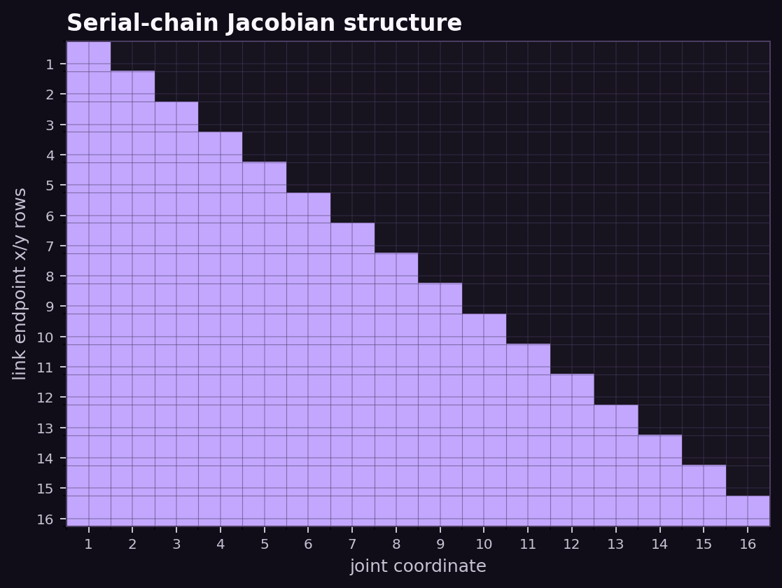
In a serial chain, joint 1 affects every downstream link. Joint 16 affects only link 16. Most relationships in a large multibody model are local, leaving predictable zeros in Jacobians and mass-matrix factorizations.

Experiment 4: predict a named site's velocity

body = sim.body_state()[0]
site = sim.site_data()["tool.tip"]

offset_world = site[:3] - body[:3]
twist = np.r_[body[7:10], body[10:13]]
J_site = np.c_[np.eye(3), -skew(offset_world)]

predicted = J_site @ twist
measured = site[7:10]

Paw-check: make the matrices answer

1. Change the box dimensions so two principal moments become equal. What happens to the uniqueness of the corresponding eigenvectors?
2. Choose a joint velocity and use $J\dot q$ to predict the two-link tip direction. Confirm it with a tiny finite step.
3. Find all elbow angles where the two-link Jacobian determinant is zero.
4. Move tool.tip to the body center. Which three columns of its point Jacobian stop contributing?
5. Count the nonzero blocks for a 100-link serial chain without allocating the full matrix.