Numerical foundations · LavenderSim

A simulator advances state

Suppose the complete state of a moving object is collected in a vector $x$ . A differential equation tells us the instantaneous rate of change:

\dot{x} = f(x,t)

For a particle, a useful state is $x=[q,v]^\mathsf{T}$ , containing position and velocity. Its derivative contains velocity and acceleration:

\frac{d}{dt}\begin{bmatrix}q\\v\end{bmatrix}=\begin{bmatrix}v\\a(q,v,t)\end{bmatrix}

The function tells us what is happening now. An integrator estimates what the state will be after a finite timestep $h$ . Every real-time simulator performs some version of this approximation.

Explicit Euler and velocity-first Euler

Explicit Euler samples the derivative at the beginning of the interval:

x_{n+1}=x_n+h f(x_n,t_n)

Applied to position and velocity, both updates use old information:

q_{n+1}=q_n+h v_n,\qquad v_{n+1}=v_n+h a_n

Semi-implicit, symplectic, or velocity-first Euler changes only the order:

v_{n+1}=v_n+h a_n,\qquad q_{n+1}=q_n+h v_{n+1}

That small change makes the position update respond to the impulse accumulated during the current step. It remains a first-order method, yet on many mechanical systems it avoids the relentless energy growth of explicit Euler.

the complete update

def semi_implicit_step(acceleration, time, position, velocity, dt):
    next_velocity = velocity + dt * acceleration(time, position, velocity)
    next_position = position + dt * next_velocity
    return next_position, next_velocity

Accuracy and stability answer different questions. Accuracy asks how closely a finite step follows the exact trajectory. Stability asks whether repeated approximation remains bounded. A high-order method can still fail when the timestep is inappropriate for the system.

Experiment 1: constant acceleration

Experiment 01verified

Measure convergence in free fall

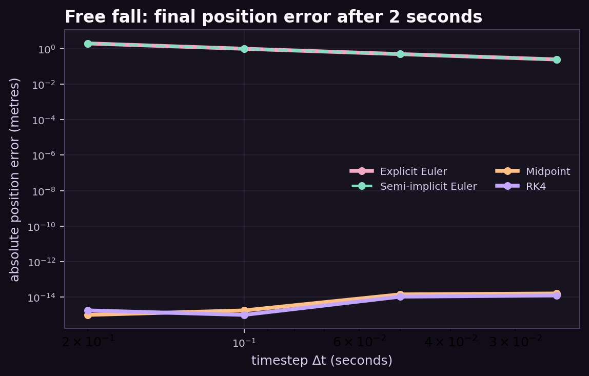
When the timestep is halved, how quickly does final position error shrink?

Drop a point from 10 metres for two seconds while ignoring the floor. Constant gravity has an exact solution, so it gives us trustworthy reference data:

q(t)=q_0+v_0t+\tfrac{1}{2}gt^2,\qquad v(t)=v_0+gt

Euler's final position error halves when $h$ halves: first-order global convergence. Midpoint and RK4 reproduce this particular constant-acceleration polynomial to floating-point roundoff. That does not mean they are exact for arbitrary dynamics.

Log plot of free-fall position error versus timestep for four integrators — The two Euler variants have equal absolute error here but opposite sign: explicit Euler falls too little, while velocity-first Euler falls too far. Their overlapping curves use different line styles.

×½Euler error after halving the timestep

O(h)Euler global error order

≈ machine εMidpoint/RK4 error for this special case

Expected result: The command exits successfully and reproduces the numerical or visual relationship described in this card.
Failure modes: Non-finite values, a reversed trend, a failed assertion, or a materially different plot means the assumptions, seed, timestep, build, or backend should be inspected before continuing.

python examples/tutorials/simulation/ch01_numerical_foundations/integrators.py --quickView source ↗

Experiment 2: energy exposes instability

Experiment 02verified

Watch an oscillator gain energy

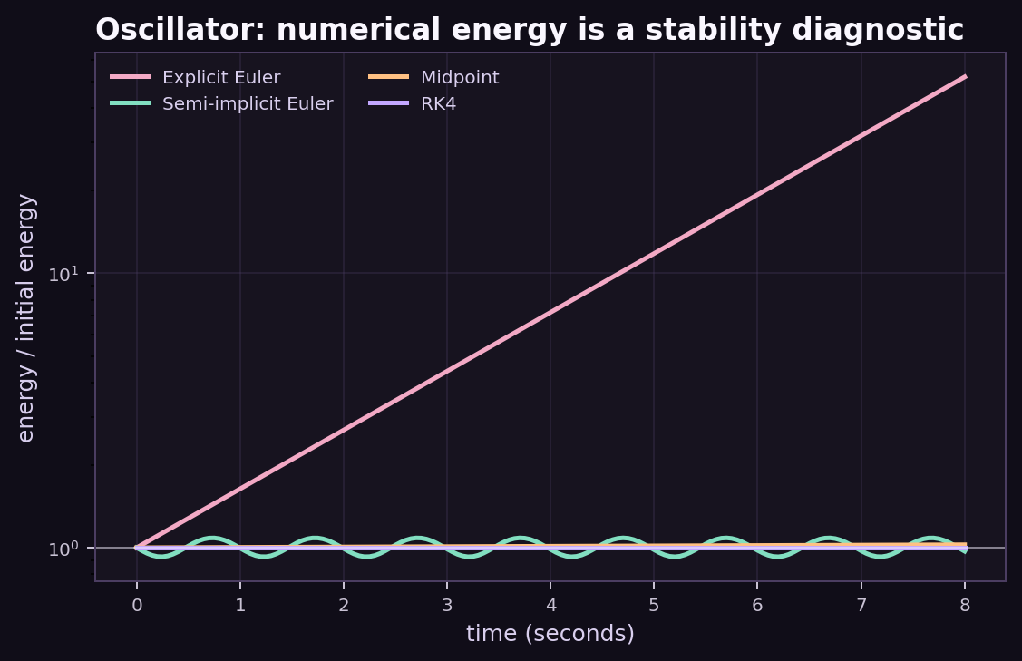
All four curves initially look plausible—so which integrator is quietly corrupting the physics?

For an ideal mass–spring oscillator, total energy should remain constant:

E=\tfrac{1}{2}m v^2+\tfrac{1}{2}kq^2

At $h=0.05\,\mathrm{s}$ , explicit Euler adds energy on every orbit. Semi-implicit Euler's energy oscillates around the correct level instead of drifting away. Midpoint drifts slowly for this setup; RK4 stays closest over the measured interval.

Energy ratio over time showing explicit Euler growth and bounded semi-implicit Euler energy — Trajectory plots can hide a growing amplitude for several cycles. Energy makes the numerical failure obvious much earlier.

>50×explicit Euler energy after 8 s

<8.6%semi-implicit maximum energy deviation

<0.004%RK4 maximum energy deviation

Expected result: The command exits successfully and reproduces the numerical or visual relationship described in this card.
Failure modes: Non-finite values, a reversed trend, a failed assertion, or a materially different plot means the assumptions, seed, timestep, build, or backend should be inspected before continuing.

python examples/tutorials/simulation/ch01_numerical_foundations/integrators.pyView source ↗

Experiment 3: timestep meets stiffness

Experiment 03verified

Map the stability boundary

Why can a controller become unstable after increasing spring stiffness without changing any other code?

The oscillator's angular frequency is $\omega=\sqrt{k/m}$ . The dimensionless product $h\omega$ compares the numerical step with the system's fastest timescale. Increasing either timestep or stiffness moves the experiment toward the bright unstable region.

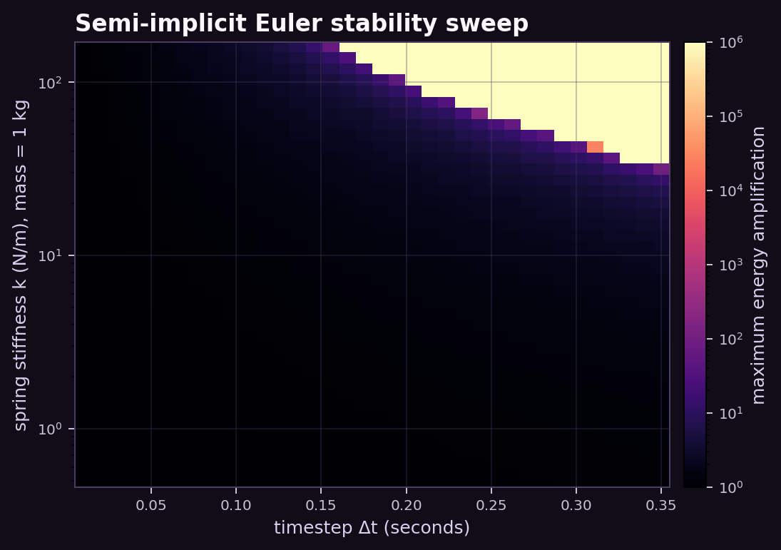
Heatmap of semi-implicit Euler energy amplification over timestep and spring stiffness — Dark cells remain near the starting energy. Bright cells amplify energy dramatically. “Use a smaller timestep” and “soften the spring” are two ways of moving away from the same boundary.

This is why stiff contacts, strong PD gains, and tiny inertias can require smaller substeps even when the policy itself only acts at 60 Hz.

Expected result: The command exits successfully and reproduces the numerical or visual relationship described in this card.
Failure modes: Non-finite values, a reversed trend, a failed assertion, or a materially different plot means the assumptions, seed, timestep, build, or backend should be inspected before continuing.

python docs-site/scripts/render_tutorial_ch01.pyView source ↗

Where LavenderSim performs the update

A LavenderSim policy can act at 60 Hz while the native engine divides each control interval into steps no larger than 1/240 second. Within a native substep, the engine:

adds gravity and external forces to velocity,
applies velocity damping,
detects and solves constraints and contacts,
updates position from the resulting velocity,
integrates and normalizes orientation.

Implemented by LavenderSim: inspect the native substep function and the 240 Hz subdivision loop. This is velocity-first integration plus constraint solving and mild damping—not the idealized gravity-only equation from Experiment 1.

observe the native body state

from lavendersim import Scene
from lavendersim.runtime import CodeSceneEnv

scene = Scene("Falling body", ground=False)
scene.sphere("ball", radius=.08, position=(0, 2, 0), mass=1)

with CodeSceneEnv(scene, control_dt=1/60) as sim:
    sim.reset(seed=1)
    for _ in range(6):
        sim.step()
        print(sim.time, sim.body_state()[0, [1, 8]])

Run the complete version with:

terminal

python examples/tutorials/simulation/ch01_numerical_foundations/lavendersim_fall.py

Observation to explain: after 0.1 seconds the ideal velocity is −0.981 m/s. LavenderSim reports approximately −0.976 m/s because its native free bodies include mild linear damping. The discrepancy is modeled engine behavior, not integration error alone.

Paw-check: change one thing

Change the oscillator timestep from 0.05 to 0.10 seconds. Predict the energy plot before running it.
Set stiffness to 160 N/m. Find a timestep where semi-implicit Euler becomes usable again.
Give the free-fall particle an initial upward velocity. Which methods remain exact to roundoff?
In lavendersim_fall.py, compare control rates of 20, 60, and 120 Hz. Explain why the native maximum substep is still 1/240 second.

What should I be able to say now?

A simulator repeatedly approximates a differential equation over a finite timestep. Explicit and semi-implicit Euler are both first order, but their long-term energy behavior can differ sharply. Stability depends on the fastest system timescale, so control frequency and native substep frequency are separate design choices.

By the end, you can…

A simulator advances state

Explicit Euler and velocity-first Euler

Experiment 1: constant acceleration

Experiment 2: energy exposes instability

Experiment 3: timestep meets stiffness

Where LavenderSim performs the update

Paw-check: change one thing