Contact mechanics

Contact is a one-sided constraint

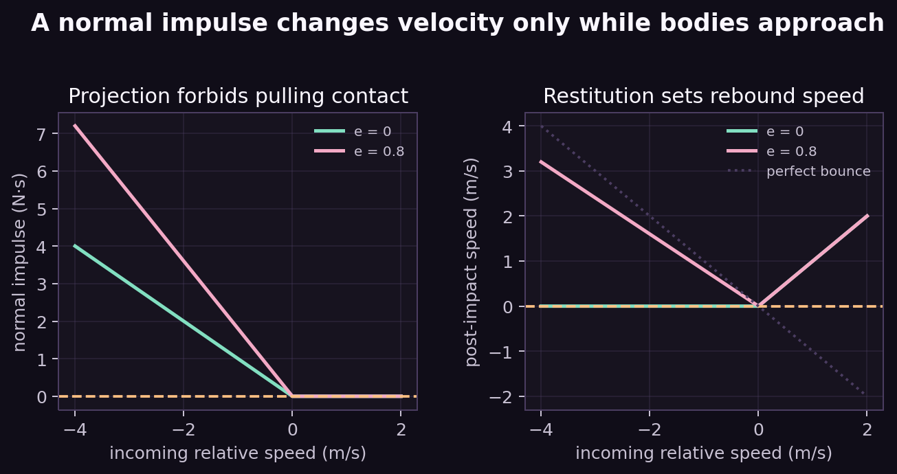
Let $\phi$ be signed separation: positive apart, zero touching, negative penetrating. Let $\lambda_n$ be the normal impulse. A normal contact may push, never pull:

This is complementarity. Separated bodies need no impulse; an active contact may produce a nonnegative impulse. A practical time-stepping solver applies the same idea to predicted normal velocity and projects every trial impulse onto $[0,\infty)$.

Experiment 1: derive the bounce impulse

An impulse $j n$ changes linear momentum instantly. For two point masses, relative normal speed changes by:

Newton's restitution law asks for $v_n^+=-e,v_n^-$ when bodies approach. Therefore:

The projection is essential. If $v_n^-\ge0$, the bodies already separate, and a negative impulse would pull them back together.

Rigid bodies can also rotate. With offsets $r_A,r_B$ from centers of mass to the contact, the scalar effective inverse mass becomes:

Replace the denominator with $k_n$. A push near a body's center is easier to translate; an off-center push must also create angular velocity.

Experiment 01verified

Implement a non-pulling impulse

What should the solver do for approaching and separating velocities?

pythonฅ

def normal_impulse(vn, inv_mass_a, inv_mass_b, restitution):
    if vn >= 0:                 # already separating
        return 0.0
    k = inv_mass_a + inv_mass_b
    return -(1 + restitution) * vn / k

Failure modes: omit relative velocity, reverse the normal without swapping body order, forget rotational effective mass, or allow $j<0$.

Expected result

The command exits successfully and reproduces the numerical or visual relationship described in this card.

Failure modes

Non-finite values, a reversed trend, a failed assertion, or a materially different plot means the assumptions, seed, timestep, build, or backend should be inspected before continuing.

python examples/tutorials/simulation/ch09_contact_mechanics/contact_mechanics.py --quickView source ↗

Experiment 2: predict a rebound

Drop from height $h$ without air resistance. Just before impact, $v^2=2gh$. Restitution multiplies speed by $e$, so energy—and therefore rebound height—scales with its square:

Experiment 02verified

Sweep restitution

Does restitution 0.8 return 80% of height?

0.64 mideal height at e = 0.8

0.659 mnative result at 480 Hz

0 N·simpulse while separating

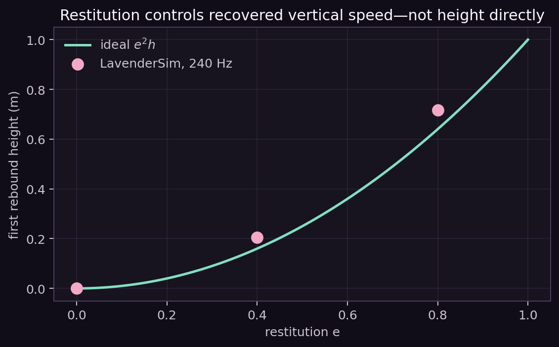
Failure modes: compare center height with surface clearance, include a later bounce in the first-apex measurement, expect $eh$, or use restitution to repair resting penetration.

Expected result

The command exits successfully and reproduces the numerical or visual relationship described in this card.

Failure modes

Non-finite values, a reversed trend, a failed assertion, or a materially different plot means the assumptions, seed, timestep, build, or backend should be inspected before continuing.

python examples/tutorials/simulation/ch09_contact_mechanics/lavendersim_drop.py --quickView source ↗

Experiment 3: separate three jobs

Restitution targets impact velocity. Stabilization adds separating velocity when numerical integration has already produced penetration. A common bias is:

where $d=-\min(\phi,0)$ is penetration. Compliance regularizes a rigid constraint into a soft one. At velocity level, LavenderSim uses $\gamma=c/\Delta t^2$:

These knobs interact. Larger steps permit deeper first overlap. Stronger stabilization may inject energy. Compliance improves conditioning and softness, but allows load-dependent deflection.

Experiment 03verified

Sweep timestep and compliance

Which error belongs to discretization, and which belongs to the chosen soft-contact model?

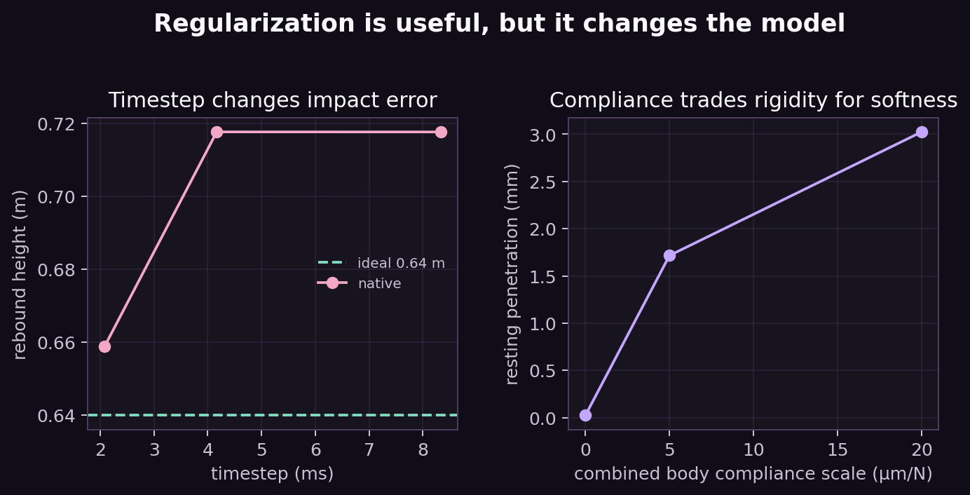
Failure modes: treat compliance as an iteration count, tune bounce with penetration bias, divide compliance by $\Delta t$ instead of $\Delta t^2$, or compare timesteps while changing simulated duration.

Expected result

The command exits successfully and reproduces the numerical or visual relationship described in this card.

Failure modes

Non-finite values, a reversed trend, a failed assertion, or a materially different plot means the assumptions, seed, timestep, build, or backend should be inspected before continuing.

python docs-site/scripts/render_tutorial_ch09.pyView source ↗

Experiment 4: inspect the contact rather than the pixels

At impact the one-kilogram sphere receives a short, large force. Once settled, its normal force approaches $mg\approx9.81$ N. LavenderSim exposes aggregate body contact data and Chapter 8's individual contact trace:

observation, reward, terminated, truncated, info = sim.step()
contacts = observation["collision"]["contacts"]
normal_force = sim.body_contact_data()[ball_id, 1]
penetration = contacts[:, 8].max() if len(contacts) else 0.0

Experiment 04verified

Plot force beside penetration

Can telemetry distinguish an impact from resting support?

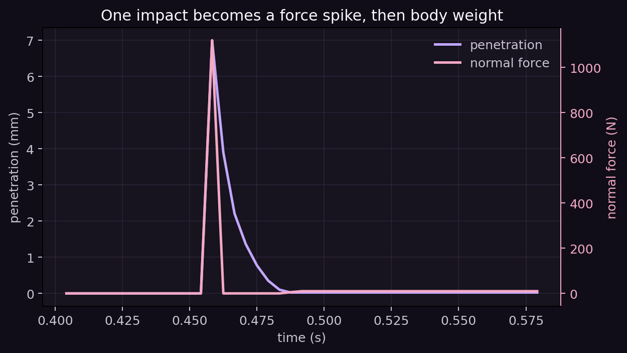
A force reported per discrete step is an average $F\approx j/\Delta t$, not a resolved microsecond material-force curve. Shorter timesteps can produce taller-looking spikes while representing a similar impulse.

Expected result

The command exits successfully and reproduces the numerical or visual relationship described in this card.

Failure modes

Non-finite values, a reversed trend, a failed assertion, or a materially different plot means the assumptions, seed, timestep, build, or backend should be inspected before continuing.

pytest -q tests/tutorials/test_ch09_contact_mechanics.pyView source ↗

Experiment 5: remember yesterday's answer

A stack has coupled contacts: changing one impulse changes another contact's velocity. Projected Gauss–Seidel visits rows repeatedly. A cold start begins with zero impulses every step. A warm start matches persistent contacts and begins from the previous step's impulses, usually close to the new solution.

Experiment 05verified

Compare cold and warm contact solves

With the same iteration budget, which initial guess leaves the smaller residual?

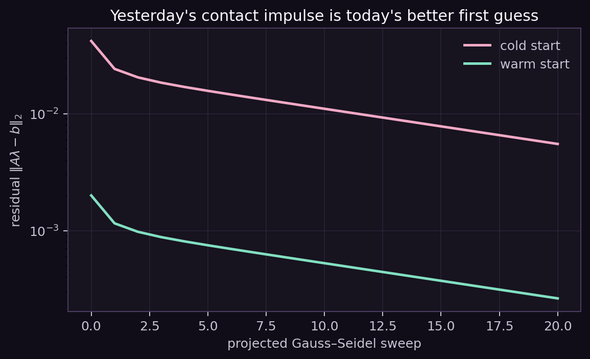
Production matching uses body pair, nearby contact point, and compatible normal. Bad matches can inject stale impulses, so caches need distance thresholds, normal checks, timestep scaling, and invalidation when topology changes.

Expected result

The command exits successfully and reproduces the numerical or visual relationship described in this card.

Failure modes

Non-finite values, a reversed trend, a failed assertion, or a materially different plot means the assumptions, seed, timestep, build, or backend should be inspected before continuing.

python examples/tutorials/simulation/ch09_contact_mechanics/contact_mechanics.pyView source ↗

The experiment found—and fixed—a real solver bug

The first native sweep initially showed identical rebound for every restitution. The contact solver recomputed the restitution condition inside each of its 22 iterations. Iteration one created a bounce; iteration two observed separation, set the bounce target to zero, and removed most of that impulse.

LavenderSim now captures the pre-solve impact velocity once when the contact is created and holds that restitution target fixed throughout the solve. The native rebound regression test protects this behavior. This is precisely why a simulator tutorial should contain quantitative experiments rather than screenshots alone.

Paw-check: make contact earn its force

1. Derive the impulse for two movable masses instead of a ball and static floor.
2. Move a contact away from a box's center and compute its rotational effective mass.
3. Set $e=1$ and plot numerical energy over five bounces.
4. Sweep stabilization gain and mark where rebound becomes artificially energetic.
5. Change the stack's load slightly and quantify the warm-start advantage.
6. Disable positional projection and measure steady penetration.
7. Compare impulse $j$ across timesteps instead of peak force.